GENROUwS

Source: GridKit/Model/PhasorDynamics/SynchronousMachine/GENROUwS/README.md

GENROU

This synchronous machine model is 6th order and is specifically designed for round rotor machines. It is a standard model used in phasor-domain industry stability studies. See the General Synchronous Machine Model for general synchronous machine information.

Notes:

• \(X_q''=X_d''\) (round rotor assumptions)

• \(X''_{d}\) does not saturate

• Same relative amount of saturation occurs on both \(d\) and \(q\) axis

Block Diagram

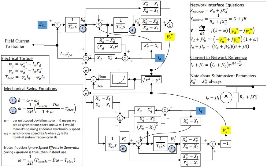
Figure 2: GENROU. Figure courtesy of PowerWorld

Model Parameters

Symbol	Units	Description	Typical Value	Note
\(P_0\)	[p.u.]	Initial active power injection	1.0
\(Q_0\)	[p.u.]	Initial reactive power injection	0.0
\(H\)	[s]	rotor inertia	3
\(D\)	[p.u.]	damping coefficient	0
\(R_a\)	[p.u.]	winding resistance	0
\(T'_{d0}\)	[s]	Open circuit direct axis transient time const.	7
\(T''_{d0}\)	[s]	Open circuit direct axis sub-transient time const.	0.04
\(T'_{q0}\)	[s]	Open circuit quadrature axis transient time const.	0.75
\(T''_{q0}\)	[s]	Open circuit quadrature axis sub-transient time const.	0.05
\(X_{d}\)	[p.u.]	Direct axis synchronous reactance	2.1
\(X'_{d}\)	[p.u.]	Direct axis transient reactance	0.2
\(X''_{d}\)	[p.u.]	Direct axis sub-transient reactance	0.18
\(X_{q}\)	[p.u.]	Quadrature axis synchronous reactance	0.5
\(X'_{q}\)	[p.u.]	Quadrature axis transient reactance	0.5
\(X''_{q}\)	[p.u.]	Quadrature axis sub-transient reactance	0.18
\(X_{\ell}\)	[p.u.]	Stator leakage reactance	0.15
\(S_{10}\)	[p.u.]	Saturation factor at 1.0 pu flux	0
\(S_{12}\)	[p.u.]	Saturation factor at 1.2 pu flux	0
\(S_\mathrm{mach}\)	[MVA]	Machine power base	100

Model Derived Parameters

\[\begin{split}\begin{aligned} G &= \dfrac{R_a}{R_a^2+(X_q'')^2} & B &= -\dfrac{X_q''}{R_a^2+(X_q'')^2}\\ S_A &= \dfrac{1.2\sqrt{S_{10}/S_{12}} +1}{\sqrt{S_{10}/S_{12}} +1} & S_B &= \dfrac{1.2\sqrt{S_{10}/S_{12}} -1}{\sqrt{S_{10}/S_{12}} -1} \\ X_{d1} &= X_d-X_d' & X_{q1} &= X_q-X_q' \\ X_{d2} &= X_d'-X_\ell & X_{q2} &= X_q'-X_\ell\\ X_{d3} &= (X_d'-X_d'')/X_{d2}^2 & X_{q3} &= (X_q'-X_q'')/X_{q2}^2 \\ X_{d4} &= (X_d'-X_d'')/X_{d2} & X_{q4} &= (X_q'-X_q'')/X_{q2} \\ X_{d5} &= (X_d''-X_\ell)/X_{d2} & X_{q5} &= (X_q''-X_\ell)/X_{q2}\\ X_{qd} &= (X_q-X_\ell)/(X_d-X_\ell) \\ f_\mathrm{base} &= f_\mathrm{sys} & S_\mathrm{mach,VA} &= 10^6 S_\mathrm{mach} \end{aligned}\end{split}\]

System bases are taken from the system at initialization.

Model Variables

Internal Variables

Differential

Symbol	Units	Description	Note
\(\delta\)	[rad]	Machine internal rotor angle
\(\omega\)	[p.u.]	Machine Speed Deviation	Optionally read by governor or stabilizer component
\(\psi'_d\)	[p.u.]	Direct axis subtransient flux
\(\psi'_q\)	[p.u.]	Quadrature axis subtransient flux
\(E'_d\)	[p.u.]	Direct axis transient flux
\(E'_q\)	[p.u.]	Quadrature axis subtransient flux

Algebraic

Symbol	Units	Description	Note
\(V_d\)	[p.u.]	Machine internal voltage, d-axis
\(V_q\)	[p.u.]	Machine internal voltage, q-axis
\(I_d\)	[p.u.]	Terminal current, d-axis
\(I_q\)	[p.u.]	Terminal current, q-axis
\(I_r\)	[p.u.]	Terminal current, real component on network reference frame	Read by bus and optionally by controllers
\(I_i\)	[p.u.]	Terminal current, imaginary component on network reference frame	Read by bus and optionally by controllers
\(\psi''_q\)	[p.u.]	Total q-axis subtransient flux
\(\psi''_d\)	[p.u.]	Total d-axis subtransient flux
\(\psi''\)	[p.u.]	Machine total subtransient flux
\(T_{e}\)	[p.u.]	Electrical torque
\(k_{sat}\)	[p.u.]	Saturation coefficient

External Variables

Differential

None.

Algebraic

Symbol	Units	Description	Note
\(V_r\)	[p.u.]	Terminal voltage, real component on network reference frame	owned by bus object
\(V_i\)	[p.u.]	Terminal voltage, imaginary component on network reference frame	owned by bus object
\(P_{m}\)	[p.u.]	Mechanical power from the prime mover	Owned by governor, constant if no governor is connected to the machine
\(E_{fd}\)	[p.u.]	Field winding voltage from the excitation system	Owned by exciter, constant if no exciter is connected to the machine

Model Equations

Differential Equations

\[\begin{split}\begin{aligned} \dot\delta &= \omega \cdot 2\pi f_\mathrm{base} \\ \dot\omega &= \dfrac{1}{2H}\left(\dfrac{P_{m}-D\omega}{1+\omega} - T_{elec}\right)\\ \dot{\psi}'_{d} &= \dfrac{1}{T''_{d0}}(E'_{q}-\psi'_{d}-X_{d2}I_{d})\\ \dot{\psi}'_{q} &= \dfrac{1}{T''_{q0}}(E'_{d}-\psi'_{q}+X_{q2}I_{q})\\ \dot{E}'_{d} &= \dfrac{1}{T'_{q0}} \left( -E'_{d}+X_{q1} (I_{q}-X_{q3}(E'_{d}-\psi'_{q}+X_{q2}I_{q})) + X_{qd}\psi''_{q}k_{sat} \right) \\ \dot{E}'_{q} &= \dfrac{1}{T'_{d0}} \left( E_{fd}-E'_{q}-X_{d1} (I_{d}+X_{d3}(E'_{q}-\psi'_{d}-X_{d2}I_{d})) -\psi''_{d}k_{sat} \right)\\ \end{aligned}\end{split}\]

Algebraic Equations

Note that for implementation purposes, some of these equations may be simplified into functions and the internal variables eliminated. Nevertheless, for modeling clarity and conformance to typical practice, the full equations are given here.

\[\begin{split}\begin{aligned} 0 &= -\psi''_{q} -E'_{d}X_{q5} - \psi'_{q}X_{q4} \\ 0 &= -\psi''_{d} +E'_{q}X_{d5} + \psi'_{d}X_{d4}\\ 0 &= -\psi'' +\sqrt{(\psi''_{d})^2+(\psi''_{q})^2} \\ 0 &= -V_{d} -\psi''_{q}(1+\omega)\\ 0 &= -V_{q} +\psi''_{d}(1+\omega)\\ 0 &= -T_{elec} +(\psi''_{d} - I_dX_d'')I_q-(\psi''_{q} - I_qX_d'')I_d \\ 0 &= -k_{sat} + S_B(\psi''-S_A)^2\sigma(\psi''-S_A) \\ 0 &= -I_d + I_r \sin(\delta) - I_i \cos(\delta) \\ 0 &= -I_q + I_r \cos(\delta) + I_i \sin(\delta) \\ 0 &= -I_r + G (V_d \sin(\delta) + V_q \cos(\delta) - V_r) - B (V_d \cos(\delta) + V_q \sin(\delta) - V_i) \\ 0 &= -I_i + B (V_d \sin(\delta) + V_q \cos(\delta) - V_r) + G (V_d \cos(\delta) + V_q \sin(\delta) - V_i) \end{aligned}\end{split}\]

Initialization

Without Saturation

Presume there is no saturation to simplify the solution procedure for the initial conditions.

Using the power-flow solution, we have explicit solutions for the following variables. The internal variables \(I_d\), \(I_q\), \(V_d\), and \(V_q\) are calculated from the network interface equations. The remaining are algebraically solved from the steady-state initial conditions.

\[\begin{split}\begin{aligned} \omega &= 0 \\ \delta &= \text{arg} \left[V_r + jV_i + (R_a + jX_q) (I_r + jI_i)\right] \\ \psi^{''}_{d} &= V_q \\ \psi^{''}_{q} &= -V_d \\ \psi^{''} &= \sqrt{(\psi''_{d})^2+(\psi''_{q})^2} \\ k_{sat} &= \begin{cases} S_B(\psi^{''}-S_A)^2, & \psi^{''} > S_A\\ 0, & \psi^{''} \le S_A \end{cases}\\ T_{elec} &= (\psi''_{d} - I_dX_d^{''})I_q-(\psi''_{q} - I_qX_d^{''})I_d \\ P_{m} &= T_{elec} \\ \psi_d' &= \psi_d'' - (X_d'' - X_\ell)I_d \\ \psi_q' &= (X_q'' - X_\ell)I_q - \psi_q'' \\ E^{'}_d &=\psi^{'}_q - X_{q2}I_q \\ E^{'}_q &=\psi^{'}_d + X_{d2}I_d \\ E_{fd} &= E'_{q}+X_{d1}I_{d}+\psi^{''}_{d}k_{sat} \\ \end{aligned}\end{split}\]

With Saturation

It is important to point out that finding the initial value of \(\delta\) for the model without saturation, the direct method can be used. In case saturation is considered, some “clever” math is needed. Key insight for determining initial \(\delta\) is that the magnitude of the saturation, which depends upon the magnitude of \(\psi''\), which is independent of \(\delta\).

\[\begin{aligned} \delta=\tan^{-1} \left[ \dfrac{(V_{i}+R_{a}I_{i})k_{sat}+(k_{sat}X''_{d}+X_{q}-X''_{q})I_{r}} {(V_{r}+R_{a}I_{r})k_{sat}-(k_{sat}X''_{d}+X_{q}-X''_{q})I_{i}} \right] \end{aligned}\]

Model Outputs

Symbol	Units	Description	Note
\(I_r\)	[p.u.]	Terminal current, real component on network reference frame	Oriented leaving the machine, system base
\(I_i\)	[p.u.]	Terminal current, imaginary component on network reference frame	Oriented leaving the machine, system base
\(P\)	[p.u.]	Active power, \(V_rI_r+V_iI_i\)	Oriented leaving the machine, system base
\(Q\)	[p.u.]	Reactive power, \(V_iI_r-V_rI_i\)	Oriented leaving the machine, system base
\(\delta\)	[rad]	Machine internal rotor angle
\(\omega\)	[p.u.]	Machine speed deviation	\(\omega=0\) at synchronous speed
\(\text{speed}\)	[p.u.]	Per-unit machine speed	\(1+\omega\)