EXDC1
Source: GridKit/Model/PhasorDynamics/Exciter/EXDC1/README.md
[!NOTE]
This documentation is not in the standard format and EXDC1 is not scheduled to be developed as of 06/26/2025.
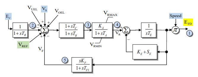
Figure 1: Exciter EXDC1 model. Figure courtesy of PoweWorld.
Nomenclature
Inputs
\(V_{REF}\) - voltage reference set point
\(E_{C}\) - output from the terminal voltage transducer
\(V_{S}\) - power system stabilizer output signal (if present)
\(V_{UEL}\) and \(V_{OEL}\) - limiters
Differential Variables
\(V_{t}\) - terminal voltage (2 is sensed \(V_{t}\))
\(V_{B}\) - input to a voltage regulator (3)
\(V_{R}\) - voltage regulator output also know as exciter field voltage (4)
\(V_{F}\) - stabilizing feedback signal (5)
Parameters
\(T_{R}\) - filter time constant, sec (0)
\(K_{A}\) - voltage regulator gain (40)
\(T_{A}\) - time constant, sec (0.1)
\(T_{B}\) - lag time constant, sec (0)
\(T_{C}\) - lead time constant, sec (0)
\(V_{RMAX}\) - maximum control element output, pu (1)
\(V_{RMIN}\) - minimum control element output, pu (-1)
\(K_{E}\) - exciter field resistance line slope margine, pu (0.1)
\(T_{E}\) - exciter time constant, sec (0.5)
\(K_{F}\) - rate feedback gain, pu (0.05)
\(T_{F1}\) - rate feedback time constant, sec (0.7)
\(E1\) - field voltage value, 1 (2.8)
\(SE1\) - saturation factor at E1, (3.7)
\(E2\) - field voltage value, 2 (3.7)
\(SE2\) - saturation factor at E2, (0.33)
Equations
First block
Second block
Third block
Fourth block
Feedback loop
Saturation is modeled using an alternative quadratic function, with the value of Se specified at two points :
same as with the synchronous machines. There are two solutions, and one where \(A<1\) should be chosen.