REECA

Source: GridKit/Model/PhasorDynamics/Converter/REECA/README.md

Renewable Energy Electrical Control Model (REECA)

REECA is a WECC renewable energy electrical control model for inverter-coupled resources. In GridKit it is represented as a signal-control model that computes active- and reactive-current commands.

Notes:

• Internal electrical quantities and current commands are on model base unless otherwise stated.

• Optional signal inputs default to their documented constant values when omitted.

• Timer-based post-dip reactive-current injection hold and active-current limit hold are not modeled in this version; \(T_{\mathrm{hld}}\) and \(T_{\mathrm{hld2}}\) must be zero.

Block Diagram

Standard REECA block diagram.

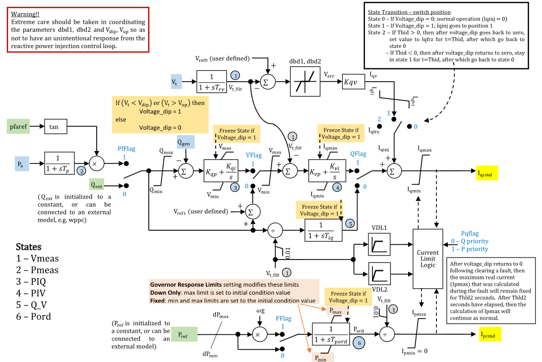
Figure 1: REECA block diagram. Figure courtesy of PowerWorld

Model Parameters

Symbol	Units	Description	Typical Value	Note
\(S^{\mathrm{base}}\)	[MVA]	REECA model power base	TBD	Block name: MVABase
\(s_{\mathrm{pf}}\)	[binary]	Power-factor control flag	TBD	Block name: PfFlag; 1 = power-factor control, 0 = Q control
\(s_V\)	[binary]	Voltage-control mode flag	TBD	Block name: VFlag; 1 = Q control, 0 = voltage control
\(s_Q\)	[binary]	Reactive-power control flag	TBD	Block name: QFlag; 1 = voltage/Q control, 0 = constant pf or Q control
\(s_P\)	[binary]	Active-power reference speed-multiplier flag	TBD	Block name: Pflag; 1 = multiply by generator speed
\(s_{PQ}\)	[binary]	P/Q priority flag for converter current limit	TBD	Block name: Pqflag; 0 = Q priority, 1 = P priority
\(T_{\mathrm{rv}}\)	[sec]	Voltage-measurement filter time constant	TBD	Block name: Trv; if zero, \(V_{\mathrm{meas}}\) is algebraic
\(T_{\mathrm{p}}\)	[sec]	Electrical-power measurement filter time constant	TBD	Block name: Tp; if zero, \(P_{\mathrm{meas}}\) is algebraic
\(V_{\mathrm{ref0}}\)	[p.u.]	Outer-loop voltage reference	TBD	Block name: Vref0; initialized to terminal voltage if omitted
\(V_{\mathrm{dip}}\)	[p.u.]	Low-voltage threshold for reactive-current injection logic	TBD	Block name: Vdip
\(V_{\mathrm{up}}\)	[p.u.]	High-voltage threshold for reactive-current injection logic	TBD	Block name: Vup
\(D_{\mathrm{bd1}}\)	[p.u.]	Overvoltage deadband for voltage-error response	TBD	Block name: dbd1
\(D_{\mathrm{bd2}}\)	[p.u.]	Undervoltage deadband for voltage-error response	TBD	Block name: dbd2
\(K_{\mathrm{qv}}\)	[p.u.]	Reactive-current injection gain during voltage dip/overvoltage logic	TBD	Block name: kqv
\(I_{\mathrm{qinj}}^{\min}\)	[p.u.]	Minimum reactive-current injection limit	TBD	Block name: Iql1
\(I_{\mathrm{qinj}}^{\max}\)	[p.u.]	Maximum reactive-current injection limit	TBD	Block name: Iqh1
\(I_{\mathrm{qinj}}^{\mathrm{frz}}\)	[p.u.]	Held reactive-current injection value after voltage dip	TBD	Block name: Iqfrz; unused when \(T_{\mathrm{hld}} = 0\)
\(T_{\mathrm{hld}}\)	[sec]	Reactive-current injection hold time after voltage dip clears	TBD	Block name: Thld; required to be zero in this version
\(Q^{\max}\)	[p.u.]	Maximum reactive-power control limit	TBD	Block name: Qmax
\(Q^{\min}\)	[p.u.]	Minimum reactive-power control limit	TBD	Block name: Qmin
\(K_{\mathrm{qp}}\)	[p.u.]	Reactive-power control proportional gain	TBD	Block name: Kqp
\(K_{\mathrm{qi}}\)	[p.u./s]	Reactive-power control integral gain	TBD	Block name: Kqi
\(V^{\max}\)	[p.u.]	Maximum voltage-control limit	TBD	Block name: Vmax
\(V^{\min}\)	[p.u.]	Minimum voltage-control limit	TBD	Block name: Vmin
\(V_{\mathrm{ref1}}\)	[p.u.]	Inner-loop voltage-control reference/bias	0	Block name: Vref1
\(K_{\mathrm{vp}}\)	[p.u.]	Voltage-control proportional gain	TBD	Block name: Kvp
\(K_{\mathrm{vi}}\)	[p.u./s]	Voltage-control integral gain	TBD	Block name: Kvi
\(T_{\mathrm{iq}}\)	[sec]	Reactive-current command lag time constant	TBD	Block name: Tiq
\(T_{\mathrm{pord}}\)	[sec]	Active-power order filter time constant	TBD	Block name: Tpord
\(R_P^{\max}\)	[p.u./s]	Positive active-power order ramp-rate limit	TBD	Block name: dPmax
\(R_P^{\min}\)	[p.u./s]	Negative active-power order ramp-rate limit	TBD	Block name: dPmin
\(P^{\max}\)	[p.u.]	Maximum active-power order limit	TBD	Block name: Pmax
\(P^{\min}\)	[p.u.]	Minimum active-power order limit	TBD	Block name: Pmin
\(I^{\max}\)	[p.u.]	Maximum total converter current	TBD	Block name: Imax
\(V_{\mathrm{q},1}\)	[p.u.]	VDL1 voltage point 1	TBD	Block name: vq1
\(I_{\mathrm{q},1}^{\max}\)	[p.u.]	VDL1 reactive-current limit point 1	TBD	Block name: lq1
\(V_{\mathrm{q},2}\)	[p.u.]	VDL1 voltage point 2	TBD	Block name: vq2
\(I_{\mathrm{q},2}^{\max}\)	[p.u.]	VDL1 reactive-current limit point 2	TBD	Block name: lq2
\(V_{\mathrm{q},3}\)	[p.u.]	VDL1 voltage point 3	TBD	Block name: vq3
\(I_{\mathrm{q},3}^{\max}\)	[p.u.]	VDL1 reactive-current limit point 3	TBD	Block name: lq3
\(V_{\mathrm{q},4}\)	[p.u.]	VDL1 voltage point 4	TBD	Block name: vq4
\(I_{\mathrm{q},4}^{\max}\)	[p.u.]	VDL1 reactive-current limit point 4	TBD	Block name: lq4
\(V_{\mathrm{p},1}\)	[p.u.]	VDL2 voltage point 1	TBD	Block name: vp1
\(I_{\mathrm{p},1}^{\max}\)	[p.u.]	VDL2 active-current limit point 1	TBD	Block name: lp1
\(V_{\mathrm{p},2}\)	[p.u.]	VDL2 voltage point 2	TBD	Block name: vp2
\(I_{\mathrm{p},2}^{\max}\)	[p.u.]	VDL2 active-current limit point 2	TBD	Block name: lp2
\(V_{\mathrm{p},3}\)	[p.u.]	VDL2 voltage point 3	TBD	Block name: vp3
\(I_{\mathrm{p},3}^{\max}\)	[p.u.]	VDL2 active-current limit point 3	TBD	Block name: lp3
\(V_{\mathrm{p},4}\)	[p.u.]	VDL2 voltage point 4	TBD	Block name: vp4
\(I_{\mathrm{p},4}^{\max}\)	[p.u.]	VDL2 active-current limit point 4	TBD	Block name: lp4
\(T_{\mathrm{hld2}}\)	[sec]	Active-current limit hold time after voltage dip clears	TBD	Block name: Thld2; required to be zero in this version

Parameter Validation

Implementations should reject invalid REECA parameter sets. If source data preprocessing adjusts active-power ramp-rate or order limits, apply these checks to the effective values used by the equations.

The required checks are:

\[\begin{split}\begin{aligned} &S^{\mathrm{base}} > 0 \\ &s_{\mathrm{pf}}, s_V, s_Q, s_P, s_{PQ} \in \{0,1\} \\ &T_{\mathrm{rv}}, T_{\mathrm{p}} \ge 0 \\ &0 \le V_{\mathrm{dip}} < V_{\mathrm{up}} \\ &D_{\mathrm{bd1}} \le 0 \le D_{\mathrm{bd2}} \\ &I_{\mathrm{qinj}}^{\min} \le I_{\mathrm{qinj}}^{\max} \\ &T_{\mathrm{hld}} = T_{\mathrm{hld2}} = 0 \\ &Q^{\min} \le Q^{\max} \\ &V^{\min} \le V^{\max} \\ &T_{\mathrm{iq}}, T_{\mathrm{pord}} > 0 \\ &R_P^{\min} < 0 < R_P^{\max} \\ &P^{\min} \le P^{\max} \\ &I^{\max} \ge 0 \\ &0 \le V_{\mathrm{q},1} < V_{\mathrm{q},2} < V_{\mathrm{q},3} < V_{\mathrm{q},4} \\ &I_{\mathrm{q},k}^{\max} \ge 0\ \text{for } k=1,\ldots,4 \\ &0 \le V_{\mathrm{p},1} < V_{\mathrm{p},2} < V_{\mathrm{p},3} < V_{\mathrm{p},4} \\ &I_{\mathrm{p},k}^{\max} \ge 0\ \text{for } k=1,\ldots,4 \end{aligned}\end{split}\]

Model Derived Parameters

The off-mode flag complements are:

\[\begin{split}\begin{aligned} s_{\mathrm{pf}}^{\mathrm{off}} &= 1 - s_{\mathrm{pf}} \\ s_V^{\mathrm{off}} &= 1 - s_V \\ s_Q^{\mathrm{off}} &= 1 - s_Q \\ s_{PQ}^{\mathrm{off}} &= 1 - s_{PQ} \end{aligned}\end{split}\]

The VDL functions use GridKit’s smooth Linear Segment helper and provide flat extrapolation outside the first and fourth voltage points:

\[\begin{split}\begin{aligned} g_q(x) &= I_{\mathrm{q},1}^{\max} + \sum_{k=1}^{3} \text{linseg}\!\left( x;\, V_{\mathrm{q},k},\, V_{\mathrm{q},k+1},\, I_{\mathrm{q},k+1}^{\max} - I_{\mathrm{q},k}^{\max} \right) \\ g_p(x) &= I_{\mathrm{p},1}^{\max} + \sum_{k=1}^{3} \text{linseg}\!\left( x;\, V_{\mathrm{p},k},\, V_{\mathrm{p},k+1},\, I_{\mathrm{p},k+1}^{\max} - I_{\mathrm{p},k}^{\max} \right) \end{aligned}\end{split}\]

Model Variables

Internal Variables

Differential

Symbol	Units	Description	Note
\(V_{\mathrm{meas}}\)	[p.u.]	Filtered terminal voltage	State 1 in Fig. 1; source label: Vmeas; algebraic when \(T_{\mathrm{rv}} = 0\)
\(P_{\mathrm{meas}}\)	[p.u.]	Filtered electrical power	State 2 in Fig. 1; source label: Pmeas; algebraic when \(T_{\mathrm{p}} = 0\)
\(x_{\mathrm{PIQ}}\)	[p.u.]	Reactive-power PI controller state	State 3 in Fig. 1; source label: PIQ
\(x_{\mathrm{PIV}}\)	[p.u.]	Voltage PI controller state	State 4 in Fig. 1; source label: PIV
\(Q_V\)	[p.u.]	Reactive-current command lag state	State 5 in Fig. 1; source label: Q_V
\(P_{\mathrm{ord}}\)	[p.u.]	Filtered active-power order	State 6 in Fig. 1; source label: Pord

Algebraic

Symbol	Units	Description	Note
\(V_T\)	[p.u.]	Terminal voltage magnitude
\(V_{\mathrm{meas}}^{\mathrm{safe}}\)	[p.u.]	Safe filtered terminal voltage for divider blocks	Lower bounded by 0.01
\(s_{\mathrm{dip}}\)	[binary]	Voltage-dip/overvoltage freeze indicator	1 when outside voltage thresholds
\(V_{\mathrm{err}}\)	[p.u.]	Deadbanded voltage error	Defined by CommonMath deadband
\(I_{\mathrm{qv}}\)	[p.u.]	Reactive-current injection candidate	Converter base
\(Q_{\mathrm{ref}}\)	[p.u.]	Selected reactive-power reference	From power-factor or external reactive-power command
\(e_Q\)	[p.u.]	Reactive-power control error	Limited \(Q_{\mathrm{ref}}\) minus \(Q_{\mathrm{gen}}\)
\(V_{\mathrm{PIQ}}\)	[p.u.]	Reactive-power control PI output	Limited by \(V^{\min}\) and \(V^{\max}\)
\(e_{\mathrm{PIV}}\)	[p.u.]	Voltage-control PI error	Selected voltage-control signal minus \(V_{\mathrm{meas}}\)
\(f_{\mathrm{pord}}\)	[p.u./s]	Active-power order derivative before ramp-rate limiting	Feeds \(r_{\mathrm{pord}}\)
\(r_{\mathrm{pord}}\)	[p.u./s]	Ramp-rate-limited active-power order derivative	Feeds \(P_{\mathrm{ord}}\) anti-windup
\(I_{\mathrm{q}}^{\mathrm{circ}}\)	[p.u.]	Reactive-current limit from converter current circle	Converter base; nonnegative algebraic branch
\(I_{\mathrm{p}}^{\mathrm{circ}}\)	[p.u.]	Active-current limit from converter current circle	Converter base; nonnegative algebraic branch
\(I_{\mathrm{q}}^{\max}\)	[p.u.]	Final reactive-current upper limit	Converter base; updated by VDL1 and current-limit logic
\(I_{\mathrm{p}}^{\max}\)	[p.u.]	Final active-current upper limit	Converter base; updated by VDL2 and current-limit logic
\(I_{\mathrm{qbase}}\)	[p.u.]	Base reactive-current command	Converter base; before \(s_Q\) selection and reactive-current injection
\(I_{\mathrm{q}}^{\mathrm{raw}}\)	[p.u.]	Raw reactive-current command before final limit	Converter base
\(I_{\mathrm{q}}^{\mathrm{cmd}}\)	[p.u.]	Reactive-current command output	Converter base
\(I_{\mathrm{p}}^{\mathrm{cmd}}\)	[p.u.]	Active-current command output	Converter base

External Variables

Differential

Symbol	Units	Description	Note
\(\omega\)	[p.u.]	Generator speed deviation	Optional, defaults to zero; source diagram \(\omega_g = 1 + \omega\)

Algebraic

Symbol	Units	Description	Note
\(V_{\mathrm{r}}\)	[p.u.]	Terminal voltage, real component	Owned by bus object
\(V_{\mathrm{i}}\)	[p.u.]	Terminal voltage, imaginary component	Owned by bus object
\(P_e\)	[p.u.]	Electrical active power	Source label: Pe
\(Q_{\mathrm{gen}}\)	[p.u.]	Reactive-power feedback	Source label: Qgen
\(Q_{\mathrm{ext}}\)	[p.u.]	External reactive-power command	Optional, defaults to initialized constant
\(\phi_{\mathrm{pf}}^{\mathrm{ref}}\)	[rad]	Power-factor angle reference	Source label: pfaref; used through tangent block
\(P_{\mathrm{ref}}\)	[p.u.]	External active-power reference	Optional, defaults to initialized constant

Model Equations

For readability, define:

\[\begin{split}\begin{aligned} f_{\mathrm{PIQ}} &= K_{\mathrm{qi}} e_Q \\ f_{\mathrm{PIV}} &= K_{\mathrm{vi}} e_{\mathrm{PIV}} \end{aligned}\end{split}\]

Differential Equations

The state-equation residuals use compact limiter notation where applicable. The measurement filters are written in descriptor form: if \(T_{\mathrm{rv}} = 0\) or \(T_{\mathrm{p}} = 0\), the corresponding variable should be tagged algebraic. The \(Q_V\) equation also uses \(T_{\mathrm{iq}}\) as a derivative coefficient, but \(T_{\mathrm{iq}} > 0\) remains required because the freeze multiplier makes the zero-time case structurally different.

\[\begin{split}\begin{aligned} 0 &= -T_{\mathrm{rv}}\dot V_{\mathrm{meas}} - V_{\mathrm{meas}} + V_T \\ 0 &= -T_{\mathrm{p}}\dot P_{\mathrm{meas}} - P_{\mathrm{meas}} + P_e \\ 0 &= -\dot x_{\mathrm{PIQ}} + (1 - s_{\mathrm{dip}}) \text{antiwindup}\!\left( V_{\mathrm{PIQ}}, f_{\mathrm{PIQ}}, V^{\min}, V^{\max} \right) \\ 0 &= -\dot x_{\mathrm{PIV}} + (1 - s_{\mathrm{dip}}) \text{antiwindup}\!\left( I_{\mathrm{qbase}}, f_{\mathrm{PIV}}, -I_{\mathrm{q}}^{\max}, I_{\mathrm{q}}^{\max} \right) \\ 0 &= -T_{\mathrm{iq}}\dot Q_V - (1 - s_{\mathrm{dip}})Q_V + (1 - s_{\mathrm{dip}})Q_{\mathrm{ref}}/V_{\mathrm{meas}}^{\mathrm{safe}} \\ 0 &= -\dot P_{\mathrm{ord}} + (1 - s_{\mathrm{dip}}) \text{antiwindup}\!\left( P_{\mathrm{ord}}, r_{\mathrm{pord}}, P^{\min}, P^{\max} \right) \end{aligned}\end{split}\]

CommonMath defines the Anti-Windup target and smooth approximation.

Algebraic Equations

The algebraic targets use CommonMath helper notation where applicable:

\[\begin{split}\begin{aligned} 0 &= -V_T^2 + V_\mathrm r^2 + V_\mathrm i^2 \\ 0 &= -V_\mathrm{meas}^\mathrm{safe} + \max(V_\mathrm{meas}, 0.01) \\ 0 &= -s_\mathrm{dip} + \text{outside}(V_T, V_\mathrm{dip}, V_\mathrm{up}) \\ 0 &= -V_\mathrm{err} + \text{deadband}(V_\mathrm{ref0} - V_\mathrm{meas}, D_\mathrm{bd1}, D_\mathrm{bd2}) \\ 0 &= -I_\mathrm{qv} + \text{clamp}(K_\mathrm{qv} V_\mathrm{err}, I_\mathrm{qinj}^{\min}, I_\mathrm{qinj}^{\max}) \\ 0 &= -Q_\mathrm{ref} + s_\mathrm{pf} P_\mathrm{meas}\tan(\phi_\mathrm{pf}^\mathrm{ref}) + s_\mathrm{pf}^\mathrm{off} Q_\mathrm{ext} \\ 0 &= -e_Q + \text{clamp}(Q_\mathrm{ref}, Q^{\min}, Q^{\max}) - Q_\mathrm{gen} \\ 0 &= -V_\mathrm{PIQ} + \text{clamp}(K_\mathrm{qp} e_Q + x_\mathrm{PIQ}, V^{\min}, V^{\max}) \\ 0 &= -e_\mathrm{PIV} + s_V V_\mathrm{PIQ} + s_V^\mathrm{off}(Q_\mathrm{ref} + V_\mathrm{ref1}) - V_\mathrm{meas} \\ 0 &= -T_\mathrm{pord} f_\mathrm{pord} + (1 + s_P\omega)P_\mathrm{ref} - P_\mathrm{ord} \\ 0 &= -r_\mathrm{pord} + \text{clamp}(f_\mathrm{pord}, R_P^{\min}, R_P^{\max}) \end{aligned}\end{split}\]

\[\begin{split}\begin{aligned} 0 &= -{I_\mathrm{q}^\mathrm{circ}}^2 + (I^{\max})^2 - s_{PQ}(I_\mathrm{p}^\mathrm{cmd})^2 \\ 0 &= -{I_\mathrm{p}^\mathrm{circ}}^2 + (I^{\max})^2 - s_{PQ}^\mathrm{off}(I_\mathrm{q}^\mathrm{cmd})^2 \\ 0 &= -I_\mathrm{q}^{\max} + \text{min}(g_q(V_\mathrm{meas}), I_\mathrm{q}^\mathrm{circ}) \\ 0 &= -I_\mathrm{p}^{\max} + \text{min}(g_p(V_\mathrm{meas}), I_\mathrm{p}^\mathrm{circ}) \\ 0 &= -I_\mathrm{qbase} + \text{clamp}(K_\mathrm{vp} e_\mathrm{PIV} + x_\mathrm{PIV}, -I_\mathrm{q}^{\max}, I_\mathrm{q}^{\max}) \\ 0 &= -I_\mathrm{q}^\mathrm{raw} + s_Q I_\mathrm{qbase} + s_Q^\mathrm{off} Q_V + s_\mathrm{dip} I_\mathrm{qv} \\ 0 &= -I_\mathrm{q}^\mathrm{cmd} + \text{clamp}(I_\mathrm{q}^\mathrm{raw}, -I_\mathrm{q}^{\max}, I_\mathrm{q}^{\max}) \\ 0 &= -I_\mathrm{p}^\mathrm{cmd} + \text{clamp}(P_\mathrm{ord}/V_\mathrm{meas}^\mathrm{safe}, 0, I_\mathrm{p}^{\max}) \end{aligned}\end{split}\]

The \(V_T\), \(I_{\mathrm{q}}^{\mathrm{circ}}\), and \(I_{\mathrm{p}}^{\mathrm{circ}}\) variables use nonnegative branches of squared algebraic residuals. This preserves the \(s_{PQ}=0\) Q-priority and \(s_{PQ}=1\) P-priority current-circle behavior without explicit square roots; a consistent solution should satisfy the nonnegative branch and nonnegative radicands.

CommonMath defines the helper targets and smooth approximations for min, max, clamp, deadband, and outside.

Initialization

Initialization is performed by evaluating the steady-state residuals in dependency order. Let subscript \(0\) denote initial values and set all internal derivatives to zero. If optional signals are not connected, use steady-state constants:

\[\begin{split}\begin{aligned} V_{T,0} &= \sqrt{V_{\mathrm{r},0}^2 + V_{\mathrm{i},0}^2} \\ \omega_0 &= 0 \\ Q_{\mathrm{ext},0} &= Q_{\mathrm{gen},0} \\ P_{\mathrm{ref},0} &= \dfrac{P_{e,0}}{1+s_P\omega_0} \end{aligned}\end{split}\]

Connected optional signals use their supplied initial values; if only some are omitted, compute the omitted constants with the connected initial values. Inconsistent supplied commands require a residual solve or initialization rejection.

If \(V_{\mathrm{ref0}}\) is omitted, set \(V_{\mathrm{ref0}} = V_{T,0}\). Initialize the measurement variables from the descriptor-form filter residuals:

\[\begin{split}\begin{aligned} V_{\mathrm{meas},0} &= V_{T,0} \\ P_{\mathrm{meas},0} &= P_{e,0} \end{aligned}\end{split}\]

When \(T_{\mathrm{rv}} = 0\) or \(T_{\mathrm{p}} = 0\), the corresponding relation is an algebraic residual rather than a differential-state initial condition.

Then evaluate the upstream algebraic chain:

\[\begin{split}\begin{aligned} V_{\mathrm{meas},0}^{\mathrm{safe}} &= \text{max}(V_{\mathrm{meas},0}, 0.01) \\ s_{\mathrm{dip},0} &= \text{outside}(V_{T,0}, V_{\mathrm{dip}}, V_{\mathrm{up}}) \\ V_{\mathrm{err},0} &= \text{deadband}(V_{\mathrm{ref0}} - V_{\mathrm{meas},0}, D_{\mathrm{bd1}}, D_{\mathrm{bd2}}) \\ I_{\mathrm{qv},0} &= \text{clamp}(K_{\mathrm{qv}} V_{\mathrm{err},0}, I_{\mathrm{qinj}}^{\min}, I_{\mathrm{qinj}}^{\max}) \\ Q_{\mathrm{ref},0} &= s_{\mathrm{pf}} P_{\mathrm{meas},0}\tan(\phi_{\mathrm{pf},0}^{\mathrm{ref}}) + s_{\mathrm{pf}}^{\mathrm{off}} Q_{\mathrm{ext},0} \\ e_{Q,0} &= \text{clamp}(Q_{\mathrm{ref},0}, Q^{\min}, Q^{\max}) - Q_{\mathrm{gen},0} \\ Q_{V,0} &= \dfrac{Q_{\mathrm{ref},0}}{V_{\mathrm{meas},0}^{\mathrm{safe}}} \\ P_{\mathrm{ord},0} &= (1+s_P\omega_0)P_{\mathrm{ref},0} \end{aligned}\end{split}\]

Initialize the reactive-power PI output so its residual and zero-derivative anti-windup condition hold:

\[\begin{split}\begin{aligned} V_{\mathrm{PIQ},0} &= \text{clamp}(K_{\mathrm{qp}} e_{Q,0} + x_{\mathrm{PIQ},0}, V^{\min}, V^{\max}) \\ e_{\mathrm{PIV},0} &= s_V V_{\mathrm{PIQ},0} + s_V^{\mathrm{off}}(Q_{\mathrm{ref},0} + V_{\mathrm{ref1}}) - V_{\mathrm{meas},0} \end{aligned}\end{split}\]

For an unsaturated zero-derivative start, require \(e_{Q,0}=0\) for \(x_{\mathrm{PIQ}}\) and choose or verify \(e_{\mathrm{PIV},0}=0\) for \(x_{\mathrm{PIV}}\). Then \(x_{\mathrm{PIQ},0}=V_{\mathrm{PIQ},0}-K_{\mathrm{qp}}e_{Q,0}\); when \(s_V=1\), set \(V_{\mathrm{PIQ},0}=V_{\mathrm{meas},0}\), and when \(s_V=0\), the supplied \(Q_{\mathrm{ref},0}+V_{\mathrm{ref1}}\) must equal \(V_{\mathrm{meas},0}\). Saturated initial conditions should be solved against the anti-windup residuals, not forced by this unsaturated formula.

Finish by evaluating \(g_q(V_{\mathrm{meas},0})\), \(g_p(V_{\mathrm{meas},0})\), and the current-limit and current-command algebraic residuals in priority order. At the command steps, use the power-flow current targets before final limiting:

\[\begin{split}\begin{aligned} I_{\mathrm{qbase},0}^{\star} &= \dfrac{Q_{\mathrm{gen},0}}{V_{\mathrm{meas},0}^{\mathrm{safe}}} \\ I_{\mathrm{p},0}^{\star} &= \dfrac{P_{\mathrm{ord},0}}{V_{\mathrm{meas},0}^{\mathrm{safe}}} \end{aligned}\end{split}\]

For \(s_{PQ}=0\), use:

\[\begin{aligned} I_{\mathrm{q},0}^{\mathrm{circ}} \rightarrow I_{\mathrm{q},0}^{\max} \rightarrow I_{\mathrm{qbase},0} \rightarrow I_{\mathrm{q},0}^{\mathrm{raw}} \rightarrow I_{\mathrm{q},0}^{\mathrm{cmd}} \rightarrow I_{\mathrm{p},0}^{\mathrm{circ}} \rightarrow I_{\mathrm{p},0}^{\max} \rightarrow I_{\mathrm{p},0}^{\mathrm{cmd}} \end{aligned}\]

For \(s_{PQ}=1\), use:

\[\begin{aligned} I_{\mathrm{p},0}^{\mathrm{circ}} \rightarrow I_{\mathrm{p},0}^{\max} \rightarrow I_{\mathrm{p},0}^{\mathrm{cmd}} \rightarrow I_{\mathrm{q},0}^{\mathrm{circ}} \rightarrow I_{\mathrm{q},0}^{\max} \rightarrow I_{\mathrm{qbase},0} \rightarrow I_{\mathrm{q},0}^{\mathrm{raw}} \rightarrow I_{\mathrm{q},0}^{\mathrm{cmd}} \end{aligned}\]

After \(I_{\mathrm{q},0}^{\max}\) and \(I_{\mathrm{qbase},0}\) are known, initialize the voltage PI state from its output residual; the unsaturated zero-derivative start also requires the \(e_{\mathrm{PIV},0}=0\) condition above:

\[x_{\mathrm{PIV},0} = I_{\mathrm{qbase},0} - K_{\mathrm{vp}} e_{\mathrm{PIV},0}\]

The current-circle variables use the nonnegative branch of the squared algebraic residuals; initialization must reject negative radicands. A standard steady-state initialization assumes \(s_{\mathrm{dip},0}=0\). If initialized during voltage-dip or overvoltage logic, \(Q_V\), \(P_{\mathrm{ord}}\), and the PI histories are not uniquely determined without the unsupported hold-timer histories, so the implementation should solve a saturation-consistent state or reject the start.

Model Outputs

Output	Units	Description	Note
iqcmd	[p.u.]	Reactive-current command output	Converter base
ipcmd	[p.u.]	Active-current command output	Converter base
vmeas	[p.u.]	Filtered terminal voltage
pmeas	[p.u.]	Filtered electrical power
piq	[p.u.]	Reactive-power PI controller state
piv	[p.u.]	Voltage PI controller state
qv	[p.u.]	Reactive-current command lag state
pord	[p.u.]	Filtered active-power order
qref	[p.u.]	Selected reactive-power reference
sdip	[binary]	Voltage-dip/overvoltage freeze indicator
iqmax	[p.u.]	Final reactive-current upper limit	Converter base
ipmax	[p.u.]	Final active-current upper limit	Converter base
iqv	[p.u.]	Reactive-current injection candidate	Converter base
vqctrl	[p.u.]	Reactive-power control PI output
iqbase	[p.u.]	Base reactive-current command	Converter base

Outstanding

Nonzero \(T_{\mathrm{hld}}\) and \(T_{\mathrm{hld2}}\) require timer/history-state support and are not modeled yet. With the required zero values, \(I_{\mathrm{qinj}}^{\mathrm{frz}}\) is unreachable and \(I_{\mathrm{p}}^{\max}\) is recalculated from VDL2 and current-circle logic at each residual evaluation instead of held after voltage recovery.

A future smooth approximation of the held reactive-current path could introduce a continuous gate \(h_q\):

\[\dot h_q = \dfrac{1}{T_{\mathrm{rise}}} s_{\mathrm{dip}}(1-h_q) - \dfrac{1}{T_{\mathrm{hld}}} (1-s_{\mathrm{dip}})h_q\]

That approximation is a modeling choice and is not part of the present equations.