IEEET1

Source: GridKit/Model/PhasorDynamics/Exciter/IEEET1/README.md

IEEE Type 1 Excitation System Model (IEEET1)

Block Diagram

Standard model of the IEEET1 Exciter.

Notes:

• \(E_C\) should be an external signal from the generator or machine, not computed through an exciter-owned Bus reference.

• The current implementation uses its Bus reference as a proxy for \(E_C\).

• This direct coupling affects numerical conditioning; production models typically use a decoupling reactance for the exciter-current path that forms \(E_C\).

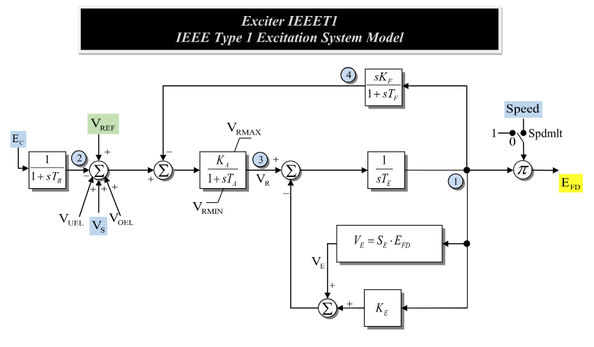
Figure 1: Exciter IEEET1 model. Figure courtesy of PowerWorld

Model Parameters

Symbol	Units	Description	Typical Value	Note
\(T_R\)	[sec]	Time constant for voltage sensing	0
\(K_A\)	[p.u.]	Coefficient for voltage regulation	50
\(T_A\)	[sec]	Time constant for voltage regulation	0.04
\(K_E\)	[p.u.]	Coefficient for excitation system	-0.06
\(T_E\)	[sec]	Time constant for excitation system	0.6
\(K_F\)	[p.u.]	Coefficient for feedback	0.09
\(T_F\)	[sec]	Time constant for feedback	1.46
\(V_R^{\min}\)	[p.u.]	Lower limit to voltage regulation	-1
\(V_R^{\max}\)	[p.u.]	Upper limit to voltage regulation	1
\(E_1\)	[p.u.]	Saturation Parameter	2.8
\(E_2\)	[p.u.]	Saturation Parameter	3.73
\(S_1\)	[p.u.]	Saturation Parameter	0.04
\(S_2\)	[p.u.]	Saturation Parameter	0.33
\(I_\text{spdlm}\)	[binary]	Speed limit flag indicator	0

Model Derived Parameters

The relationship of the derived parameters is defined by the following quadratic model. The parameters are chosen so that the quadratic model represents the expected saturation near the operating region.

\[\begin{split}\begin{aligned} S_1 &= S_B(E_1-S_A)^2 \\ S_2 &= S_B(E_2-S_A)^2 \\ \end{aligned}\end{split}\]

Generally, this system has two solutions. The non-extraneous solution is as follows.

\[\begin{split}\begin{aligned} C &= \sqrt{ \dfrac {S_2} {S_1} } \\ S_A &= \dfrac {C E_1 - E_2} {C - 1} \\ S_B &= \dfrac {S_1} {(E_1-S_A)^2} \end{aligned}\end{split}\]

Model Variables

Internal Variables

Differential

Symbol	Units	Description	Note
\(V_{ts}\)	[p.u.]	Sensed terminal voltage
\(V_R\)	[p.u.]	Voltage regulator
\(E_{fd}'\)	[p.u.]	Field-current pre-speed multiplier
\(V_{fx}\)	[p.u.]	Exciter feedback internal state

Algebraic

Symbol	Units	Description	Note
\(V_{tr}\)	[p.u.]	Terminal Voltage Error
\(V_f\)	[p.u.]	Feedback Voltage
\(V_E\)	[p.u.]	Excitation control voltage
\(E_{fd}\)	[p.u.]	Field winding voltage
\(k_\text{sat}\)	[p.u.]	Saturation variable

External Variables

Differential

Symbol	Units	Description	Note
\(\omega\)	[p.u.]	Machine Speed Deviation	Read from a Machine Model

Algebraic

Symbol	Units	Description	Note
\(E_C\)	[p.u.]	Compensated machine terminal voltage magnitude
\(V_\text{ref}\)	[p.u.]	Reference terminal voltage
\(V_{UEL}\)	[p.u.]	Input from under excitation limiter
\(V_{OEL}\)	[p.u.]	Input from over excitation limiter
\(V_S\)	[p.u.]	Input from stabilizer controller

Model Equations

Differential Equations

The IEEET1 differential equations, as derived from the model diagram. Define the pre-limit derivative of \(V_R\)

\[f = \dfrac{1}{T_A}\left[-V_R + K_A V_{tr}\right]\]

so that \(\dot V_R\) is the anti-windup limited derivative.

\[\begin{split}\begin{aligned} \dot V_{ts} &= \dfrac{1}{T_R}(E_C-V_{ts}) \\ \dot V_R &= \text{antiwindup} \left(V_R, f;\ V_R^{\min}, V_R^{\max}\right) \\ \dot E_{fd}' &= \dfrac{1}{T_E}(V_R-V_E-K_E E_{fd}') \\ \dot V_{fx} &= \dfrac{1}{T_F}V_f \\ \end{aligned}\end{split}\]

CommonMath defines the Anti-Windup target and smooth approximation.

Algebraic Equations

The algebraic equations of the exciter.

\[\begin{split}\begin{aligned} V_{tr} &= V_\text{ref} +V_{UEL} + V_{OEL} + V_S - V_f- V_{ts}\\ V_f &= \dfrac{E_{fd}' K_F}{T_F} - V_{fx}\\ V_E &= k_\text{sat}\cdot E_{fd}' \\ E_{fd}&= \begin{cases} (1+\omega)E_{fd}' & \text{if } I_\text{spdlm}=1\\ E_{fd}' & \text{else} \\ \end{cases}\\ k_\text{sat}&= \begin{cases} S_B(E_{fd}' -S_A)^2 & \text{if } E_{fd}' >S_A\\ 0 & \text{else } \\ \end{cases} \\ \end{aligned}\end{split}\]

Smooth Piecewise Approximation (Algebraic)

For the algebraic piecewise functions (non-flags), this implementation is straightforward when the approximation above is used. Here \(q\) is GridKit’s Quadratic Ramp.

\[\begin{split}\begin{aligned} E_{fd} &=(1 + \omega I_\text{spdlm})E_{fd}' \\ k_\text{sat} &=S_B\, q(E_{fd}' -S_A) \end{aligned}\end{split}\]

Initialization

The machine initializes \(E_{fd}\) first. IEEET1 reads that value as \(E_{fd,0}\), along with any attached \(\omega\) and \(V_S\), and solves the steady-state algebraic chain so all residuals vanish with \(\dot y = 0\). There is no compensation impedance, so \(E_C\) is taken as the terminal voltage magnitude. Saturation and the speed-limit flag are included directly; \(V_\text{ref}\) is set to close the \(V_{tr}\) equation with the current auxiliary inputs.

\[\begin{split}\begin{aligned} E_C &= \sqrt{V_r^2 + V_i^2} \\ E_{fd}' &= \dfrac{E_{fd,0}}{1 + I_\text{spdlm}\,\omega} \\ k_\text{sat} &= S_B\, q(E_{fd}' - S_A) \\ V_E &= k_\text{sat}\, E_{fd}' \\ V_R &= K_E\, E_{fd}' + V_E \\ V_{tr} &= \dfrac{V_R}{K_A} \\ V_{fx} &= \dfrac{K_F}{T_F}\, E_{fd}' \\ V_{ts} &= E_C \\ V_f &= 0 \\ V_\text{ref} &= E_C + V_{tr} - V_{UEL} - V_{OEL} - V_S \end{aligned}\end{split}\]

All internal derivatives initialize to zero.

Model Outputs

The field voltage, \(E_{fd}\), is an internal model variable.

The magnetic saturation coefficient \(k_\text{sat}\) is calculated from \(E_{fd}\) using the smooth piecewise version above.