REGCA

Source: GridKit/Model/PhasorDynamics/Converter/REGCA/README.md

Renewable Energy Generator/Converter Model (REGCA)

REGCA is a first-generation WECC renewable generator/converter model for inverter-coupled resources. In GridKit it is represented as a controlled current source at the network interface.

Notes:

• LVACM uses the unfiltered terminal voltage \(V_T\); LVPL uses the filtered voltage \(V_M\).

• Internal currents are on converter base; bus injections are converted to system base in the network interface.

• HVRCM is represented by internal algebraic current \(I_{\mathrm{q}}^{\mathrm{extra}}\).

Block Diagram

Standard REGCA converter-interface model.

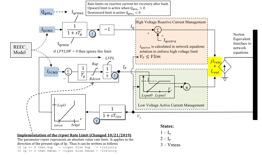
Figure 1: Generator/Converter REGCA model. Figure courtesy of PowerWorld

Model Parameters

Symbol	Units	Description	Typical Value	Note
\(P_{\mathrm{0}}\)	[p.u.]	Initial active power injection		On system base
\(Q_{\mathrm{0}}\)	[p.u.]	Initial reactive power injection		On system base
\(S^{\mathrm{conv}}\)	[MVA]	Converter/model power base	TBD
\(T_{\mathrm{g}}\)	[sec]	Converter current-control lag time constant	TBD
\(T_M\)	[sec]	Terminal voltage sensor time constant	TBD	Block name: Tfltr
\(R_{\mathrm{q}}^{\max}\)	[p.u./s]	Reactive-current recovery positive rate limit	TBD	Block name: Iqrmax
\(R_{\mathrm{q}}^{\min}\)	[p.u./s]	Reactive-current recovery negative rate limit	TBD	Block name: Iqrmin
\(R_{\mathrm{p}}^{\max}\)	[p.u./s]	Active-current magnitude recovery rate limit	TBD	Block name: rrpwr
\(s_L\)	[binary]	LVPL switch	TBD	Block name: LPVLSW
\(I_{L1}\)	[p.u.]	LVPL upper-current ceiling	TBD	Block name: Lvpl1
\(V_{L0}\)	[p.u.]	LVPL zero-crossing voltage	TBD	Block name: xerox
\(V_{L1}\)	[p.u.]	LVPL upper breakpoint voltage	TBD	Block name: brkpt
\(V_{A0}\)	[p.u.]	LVACM lower breakpoint voltage	TBD	Block name: Lvpnt0
\(V_{A1}\)	[p.u.]	LVACM upper breakpoint voltage	TBD	Block name: Lvpnt1
\(V_{\mathrm{hv}}^{\max}\)	[p.u.]	Terminal-voltage ceiling for HV reactive management	TBD	Block name: Vlim

Parameter Validation

Implementations should reject or report invalid parameter sets:

\[\begin{split}\begin{aligned} S^{\mathrm{conv}} &> 0 & T_{\mathrm{g}} &> 0 & T_M &> 0 \\ R_{\mathrm{p}}^{\max} &> 0 & R_{\mathrm{q}}^{\min} &< 0 < R_{\mathrm{q}}^{\max} & s_L &\in \{0,1\} \\ I_{L1} &\ge 0 & 0 &\le V_{L0} < V_{L1} & 0 &\le V_{A0} < V_{A1} \\ V_{\mathrm{hv}}^{\max} &> 0 \end{aligned}\end{split}\]

Model Derived Parameters

The smooth active-current bound equations use \(M_{\mathrm{p}}\), a numerical relaxation for inactive \(\pm\infty\) rate bounds:

\[M_{\mathrm{p}} = 100 R_{\mathrm{p}}^{\max}\]

\(M_{\mathrm{p}}\) is not a physical REGCA parameter; it should be large enough that inactive bounds do not bind expected \(f_{\mathrm{p}}\) values while staying moderate enough to keep the smooth clamp well conditioned.

Model Variables

Internal Variables

Differential

Symbol	Units	Description	Note
\(V_M\)	[p.u.]	Filtered terminal voltage	State 3 in Fig. 1
\(I_{\mathrm{q}}\)	[p.u.]	Reactive-current state	State 1 in Fig. 1 before the -1 block; converter base
\(I_{\mathrm{p}}\)	[p.u.]	Active-current state	State 2 in Fig. 1; converter base

Algebraic

Symbol	Units	Description	Note
\(V_T\)	[p.u.]	Terminal voltage magnitude
\(I_{\mathrm{i}}\)	[p.u.]	Injected current, imaginary component on network reference frame	Converter base
\(I_{\mathrm{q}}^{\mathrm{extra}}\)	[p.u.]	Extra inductive current from high-voltage reactive current management	Converter base
\(I_L\)	[p.u.]	LVPL upper-limit current curve	Function of \(V_M\)
\(I_{\mathrm{r}}\)	[p.u.]	Injected current, real component on network reference frame	Converter base
\(\ell_{\mathrm{p}}\)	[p.u./s]	Smooth active-current lower rate bound	Equivalent to diagram Rdown
\(u_{\mathrm{p}}\)	[p.u./s]	Smooth active-current upper rate bound	Effective Rup; includes LVPL anti-windup when \(s_L=1\)

External Variables

Differential

None.

Algebraic

Symbol	Units	Description	Note
\(V_{\mathrm{r}}\)	[p.u.]	Terminal voltage, real component on network reference frame	Owned by bus object
\(V_{\mathrm{i}}\)	[p.u.]	Terminal voltage, imaginary component on network reference frame	Owned by bus object
\(I_{\mathrm{q}}^{\mathrm{cmd}}\)	[p.u.]	Reactive-current command	Converter base; owned by REEC, constant if no REEC is connected
\(I_{\mathrm{p}}^{\mathrm{cmd}}\)	[p.u.]	Active-current command	Converter base; owned by REEC, constant if no REEC is connected

Model Equations

Define the pre-limit current derivatives:

\[\begin{split}\begin{aligned} f_{\mathrm{q}} &= \dfrac{1}{T_{\mathrm{g}}}(I_{\mathrm{q}}^{\mathrm{cmd}} - I_{\mathrm{q}}) \\ f_{\mathrm{p}} &= \dfrac{1}{T_{\mathrm{g}}}(I_{\mathrm{p}}^{\mathrm{cmd}} - I_{\mathrm{p}}) \end{aligned}\end{split}\]

Differential Equations

The exact state equations are

\[\begin{split}\begin{aligned} 0 &= -T_M \dot V_M - V_M + V_T \\ 0 &= -\dot I_{\mathrm{q}} + \begin{cases} \min(f_{\mathrm{q}}, R_{\mathrm{q}}^{\max}) & Q_{\mathrm{0}} > 0 \\ \max(f_{\mathrm{q}}, R_{\mathrm{q}}^{\min}) & Q_{\mathrm{0}} \le 0 \end{cases} \\ 0 &= -\dot I_{\mathrm{p}} + \text{clamp}(f_{\mathrm{p}}, \ell_{\mathrm{p}}, u_{\mathrm{p}}) \end{aligned}\end{split}\]

The implemented smooth state equations are

\[\begin{split}\begin{aligned} 0 &= -T_M \dot V_M - V_M + V_T \\ 0 &= -\dot I_{\mathrm{q}} + \begin{cases} f_{\mathrm{q}} - \rho(f_{\mathrm{q}} - R_{\mathrm{q}}^{\max}) & Q_{\mathrm{0}} > 0 \\ f_{\mathrm{q}} + \rho(R_{\mathrm{q}}^{\min} - f_{\mathrm{q}}) & Q_{\mathrm{0}} \le 0 \end{cases} \\ 0 &= -\dot I_{\mathrm{p}} + \ell_{\mathrm{p}} + \rho(f_{\mathrm{p}} - \ell_{\mathrm{p}}) - \rho(f_{\mathrm{p}} - u_{\mathrm{p}}) \end{aligned}\end{split}\]

Here \(\rho\) is GridKit’s smooth ramp function. The \(I_{\mathrm{q}}\) branch is selected by initial reactive power \(Q_{\mathrm{0}}\). The \(I_{\mathrm{p}}\) equation is the smooth clamp of \(f_{\mathrm{p}}\) between the algebraic bounds \(\ell_{\mathrm{p}}\) and \(u_{\mathrm{p}}\).

Algebraic Equations

The piecewise definitions in this section switch on continuous states, unlike the \(I_{\mathrm{q}}\) differential branch selected by initial conditions. The exact algebraic targets are:

\[\begin{split}\begin{aligned} 0 &= -V_T^2 + V_{\mathrm{r}}^2 + V_{\mathrm{i}}^2 \\ I_{\mathrm{i}} &= -I_{\mathrm{q}} + I_{\mathrm{q}}^{\mathrm{extra}} \\ 0 &= \begin{cases} I_{\mathrm{q}}^{\mathrm{extra}} & V_T < V_{\mathrm{hv}}^{\max} \\ V_T - V_{\mathrm{hv}}^{\max} & I_{\mathrm{q}}^{\mathrm{extra}} > 0 \end{cases} \\ I_L &= I_{L1} \begin{cases} 0 & V_M \le V_{L0} \\ \dfrac{V_M - V_{L0}}{V_{L1} - V_{L0}} & V_{L0} < V_M < V_{L1} \\ 1 & V_M \ge V_{L1} \end{cases} \\ I_{\mathrm{r}} &= I_{\mathrm{p}} \begin{cases} 0 & V_T \le V_{A0} \\ \dfrac{V_T - V_{A0}}{V_{A1} - V_{A0}} & V_{A0} < V_T < V_{A1} \\ 1 & V_T \ge V_{A1} \end{cases} \\ \ell_{\mathrm{p}} &= \begin{cases} -R_{\mathrm{p}}^{\max} & I_{\mathrm{p}} \le 0 \\ -\infty & I_{\mathrm{p}} > 0 \end{cases} \\ u_{\mathrm{p}} &= \begin{cases} R_{\mathrm{p}}^{\max} & I_{\mathrm{p}} \ge 0 \ \land\ (s_L = 0 \lor I_{\mathrm{p}} < I_L) \\ 0 & s_L = 1 \ \land\ I_{\mathrm{p}} \ge I_L \\ \infty & I_{\mathrm{p}} < 0 \end{cases} \end{aligned}\end{split}\]

The implemented algebraic residuals use smooth \(\text{linseg}\), \(\rho\), and \(\sigma\) operators:

\[\begin{split}\begin{aligned} 0 &= -V_T^2 + V_{\mathrm{r}}^2 + V_{\mathrm{i}}^2 \\ 0 &= -I_{\mathrm{i}} - I_{\mathrm{q}} + I_{\mathrm{q}}^{\mathrm{extra}} \\ 0 &= -I_{\mathrm{q}}^{\mathrm{extra}} + \rho\!\left(I_{\mathrm{q}}^{\mathrm{extra}} - (V_{\mathrm{hv}}^{\max} - V_T)\right) \\ 0 &= -I_L + \text{linseg}(V_M;\ V_{L0},\ V_{L1},\ I_{L1}) \\ 0 &= -I_{\mathrm{r}} + I_{\mathrm{p}}\text{linseg}(V_T;\ V_{A0},\ V_{A1},\ 1) \\ 0 &= -\ell_{\mathrm{p}} - R_{\mathrm{p}}^{\max} - (M_{\mathrm{p}} - R_{\mathrm{p}}^{\max})\sigma(I_{\mathrm{p}}) \\ 0 &= -u_{\mathrm{p}} + \begin{cases} M_{\mathrm{p}}(1-\sigma(I_{\mathrm{p}})) + R_{\mathrm{p}}^{\max}\sigma(I_{\mathrm{p}}) \sigma(I_L - I_{\mathrm{p}}) & s_L = 1 \\ M_{\mathrm{p}}(1-\sigma(I_{\mathrm{p}})) + R_{\mathrm{p}}^{\max}\sigma(I_{\mathrm{p}}) & s_L = 0 \end{cases} \end{aligned}\end{split}\]

The \(V_T\) residual is kept in squared form for smoothness at the origin.

Network Interface

The bus receives system-base current injections converted from converter-base REGCA currents:

\[\begin{split}\begin{aligned} I_{\mathrm{r}}^{\mathrm{inj}} &:= I_{\mathrm{r}}\dfrac{S^{\mathrm{conv}}}{S^{\mathrm{sys}}} \\ I_{\mathrm{i}}^{\mathrm{inj}} &:= I_{\mathrm{i}}\dfrac{S^{\mathrm{conv}}}{S^{\mathrm{sys}}} \end{aligned}\end{split}\]

Positive current injection is into the bus.

Initialization

Given initialized bus voltage \(V_{\mathrm{r}}, V_{\mathrm{i}}\), compute the steady-state initial values:

\[\begin{split}\begin{aligned} V_T &= \sqrt{V_\mathrm{r}^2 + V_\mathrm{i}^2} \\ I_\mathrm{r0} &= \dfrac{P_0 V_\mathrm{r} + Q_0 V_\mathrm{i}}{V_T^2} \dfrac{S^\mathrm{sys}}{S^\mathrm{conv}} \\ I_\mathrm{i0} &= \dfrac{P_0 V_\mathrm{i} - Q_0 V_\mathrm{r}}{V_T^2} \dfrac{S^\mathrm{sys}}{S^\mathrm{conv}} \\ V_{M0} &= V_T \\ I_{L0} &= \text{linseg}(V_T;\ V_{L0},\ V_{L1},\ I_{L1}) \\ I_\mathrm{p0} &= \dfrac{I_\mathrm{r0}} {\text{linseg}(V_T;\ V_{A0},\ V_{A1},\ 1)} \\ \ell_\mathrm{p0} &= -R_\mathrm{p}^{\max} - (M_\mathrm{p} - R_\mathrm{p}^{\max})\sigma(I_\mathrm{p0}) \\ u_\mathrm{p0} &= \begin{cases} M_\mathrm{p}(1-\sigma(I_\mathrm{p0})) + R_\mathrm{p}^{\max}\sigma(I_\mathrm{p0}) \sigma(I_{L0} - I_\mathrm{p0}) & s_L = 1 \\ M_\mathrm{p}(1-\sigma(I_\mathrm{p0})) + R_\mathrm{p}^{\max}\sigma(I_\mathrm{p0}) & s_L = 0 \end{cases} \\ I_\mathrm{q0}^\mathrm{extra} &= 0 \\ I_\mathrm{q0} &= -I_\mathrm{i0} + I_\mathrm{q0}^\mathrm{extra} \\ I_\mathrm{p0}^\mathrm{cmd} &= I_\mathrm{p0} \\ I_\mathrm{q0}^\mathrm{cmd} &= I_\mathrm{q0} \end{aligned}\end{split}\]

For normal power-flow starts, \(V_T > V_{A1}\), so \(\text{linseg}(V_T;\ V_{A0},\ V_{A1},\ 1) = 1\) and the \(I_{\mathrm{p0}}\) formula is well defined.

Initialization should verify:

• \(V_T \le V_{\mathrm{hv}}^{\max}\). If \(V_T \ge V_{\mathrm{hv}}^{\max}\), \(I_{\mathrm{q0}}^{\mathrm{extra}} = 0\) may not satisfy the HVRCM algebraic condition, and a nonzero value should be solved or the initialization rejected.

• \(\text{linseg}(V_T;\ V_{A0},\ V_{A1},\ 1) > 0\) when \(I_{\mathrm{r0}} \ne 0\). If the LVACM gain is zero, no finite \(I_{\mathrm{p0}}\) can reproduce nonzero initial active current.

All internal derivatives initialize to zero.

Model Outputs

Real and imaginary injected currents, \(I_{\mathrm{r}}\) and \(I_{\mathrm{i}}\), are converter-base algebraic variables. System-base power outputs use the bus-facing currents:

\[\begin{split}\begin{aligned} P &= V_{\mathrm{r}} I_{\mathrm{r}}^{\mathrm{inj}} + V_{\mathrm{i}} I_{\mathrm{i}}^{\mathrm{inj}} \\ Q &= V_{\mathrm{i}} I_{\mathrm{r}}^{\mathrm{inj}} - V_{\mathrm{r}} I_{\mathrm{i}}^{\mathrm{inj}} \end{aligned}\end{split}\]

Power outputs are positive leaving the converter and entering the bus.