Branch

Source: GridKit/Model/PhasorDynamics/Branch/README.md

Branch Model

The Branch model represents a two-terminal phasor-domain \(\pi\) branch with an optional off-nominal tap magnitude and phase shift on bus 1. Terminal current contributions are oriented entering the adjacent buses.

Notes:

• Setting \(\tau = 1\) and \(\theta = 0\) gives the ordinary symmetric transmission-line \(\pi\) model.

• \(G\) and \(B\) are total branch shunt values split equally between terminals.

• The branch has no solver-owned variables; it contributes current residuals directly to the connected buses.

Circuit Diagram

An ideal complex tap is placed on the bus-1 side of the branch equivalent. The ordinary transmission-line \(\pi\) model is recovered with \(\tau = 1\) and \(\theta = 0\).

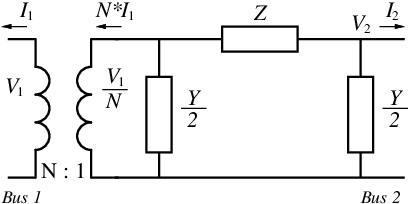
Figure 1: Branch equivalent circuit

Model Parameters

Symbol	Units	Description	Typical Value	Note
\(R\)	[p.u.]	Branch series resistance
\(X\)	[p.u.]	Branch series reactance
\(G\)	[p.u.]	Total branch shunt conductance	0
\(B\)	[p.u.]	Total branch shunt susceptance	0
\(\tau\)	[p.u.]	Off-nominal tap magnitude on bus-1 side	1	Parameter name: tap
\(\theta\)	[rad]	Phase-shift angle	0	Parameter name: phase

Parameter Validation

Invalid Branch parameter sets are rejected by the following checks:

\[\begin{split}\begin{aligned} &R, X, G, B, \tau, \theta \in \mathbb{R}\ \text{and finite} \\ &R^2 + X^2 > 0 \\ &\tau > 0 \end{aligned}\end{split}\]

Model Derived Parameters

The series and shunt admittances are:

\[\begin{split}\begin{aligned} Y_{\mathrm{br}} &= \dfrac{1}{R + jX} \\ Y_{\mathrm{sh}} &= G + jB \end{aligned}\end{split}\]

The nominal \(\pi\)-branch admittance matrix is the sum of the series and shunt admittance contributions:

\[\begin{split}\begin{aligned} \mathbf{Y}_0 &= \begin{bmatrix} -Y_{\mathrm{br}} & Y_{\mathrm{br}} \\ Y_{\mathrm{br}} & -Y_{\mathrm{br}} \end{bmatrix} + \dfrac{1}{2} \begin{bmatrix} -Y_{\mathrm{sh}} & 0 \\ 0 & -Y_{\mathrm{sh}} \end{bmatrix} \end{aligned}\end{split}\]

The off-nominal transformer transformation uses bus 1 as the tap side:

\[\begin{split}\begin{aligned} \mathbf{M} &= \begin{bmatrix} \tau^{-1} & 0 \\ 0 & e^{j\theta} \end{bmatrix} \\ \mathbf{Y} &= \mathbf{M}^{\dagger}\mathbf{Y}_0\mathbf{M} \end{aligned}\end{split}\]

For the equations below, write each entry as \(Y_{mn}=G_{mn}+jB_{mn}\).

Model Variables

Internal Variables

Differential

None.

Algebraic

None.

External Variables

Differential

None.

Algebraic

Symbol	Units	Description	Note
\(V_{r1}\)	[p.u.]	Terminal voltage, real component, bus 1	Owned by bus object
\(V_{i1}\)	[p.u.]	Terminal voltage, imaginary component, bus 1	Owned by bus object
\(V_{r2}\)	[p.u.]	Terminal voltage, real component, bus 2	Owned by bus object
\(V_{i2}\)	[p.u.]	Terminal voltage, imaginary component, bus 2	Owned by bus object

Model Equations

Differential Equations

None.

Algebraic Equations

The branch current relation is \(0 = -\mathbf{I} + \mathbf{Y}\mathbf{V}\).

\[\begin{split}\begin{aligned} I_{r1} &= G_{11} V_{r1} - B_{11} V_{i1} + G_{12} V_{r2} - B_{12} V_{i2} \\ I_{i1} &= B_{11} V_{r1} + G_{11} V_{i1} + B_{12} V_{r2} + G_{12} V_{i2} \\ I_{r2} &= G_{21} V_{r1} - B_{21} V_{i1} + G_{22} V_{r2} - B_{22} V_{i2} \\ I_{i2} &= B_{21} V_{r1} + G_{21} V_{i1} + B_{22} V_{r2} + G_{22} V_{i2} \end{aligned}\end{split}\]

These current contributions are added to the connected bus residuals with positive sign because branch current is oriented entering the bus.

Initialization

The Branch model has no internal state to initialize. During construction or parameter updates, the component computes \(\mathbf{Y}\) from the current parameter values. Initial terminal current and power monitor values are evaluated from the connected bus voltages. Parameter verification rejects the invalid cases listed above.

Model Outputs

Output	Units	Description	Note
ir1	[p.u.]	Terminal current, real component, bus 1	Oriented entering bus 1
ii1	[p.u.]	Terminal current, imaginary component, bus 1	Oriented entering bus 1
im1	[p.u.]	Terminal current magnitude, bus 1
p1	[p.u.]	Active power at bus 1 terminal	Positive entering bus 1
q1	[p.u.]	Reactive power at bus 1 terminal	Positive entering bus 1
ir2	[p.u.]	Terminal current, real component, bus 2	Oriented entering bus 2
ii2	[p.u.]	Terminal current, imaginary component, bus 2	Oriented entering bus 2
im2	[p.u.]	Terminal current magnitude, bus 2
p2	[p.u.]	Active power at bus 2 terminal	Positive entering bus 2
q2	[p.u.]	Reactive power at bus 2 terminal	Positive entering bus 2

Current magnitudes are:

\[\begin{split}\begin{aligned} I_{m1} &= \sqrt{I_{r1}^2 + I_{i1}^2} \\ I_{m2} &= \sqrt{I_{r2}^2 + I_{i2}^2} \end{aligned}\end{split}\]

Complex power at each end is defined as \(S=VI^{\ast}\):

\[\begin{split}\begin{aligned} P_1 &= V_{r1} I_{r1} + V_{i1} I_{i1} \\ Q_1 &= V_{i1} I_{r1} - V_{r1} I_{i1} \\ P_2 &= V_{r2} I_{r2} + V_{i2} I_{i2} \\ Q_2 &= V_{i2} I_{r2} - V_{r2} I_{i2} \end{aligned}\end{split}\]