IEEET1

Block Diagram

Standard model of the IEEET1 Exciter.

Notes:

The voltage-sensing input currently uses the positive bus-voltage magnitude \(\sqrt{V_r^2 + V_i^2}\); a separate compensation-impedance path is not modeled here.

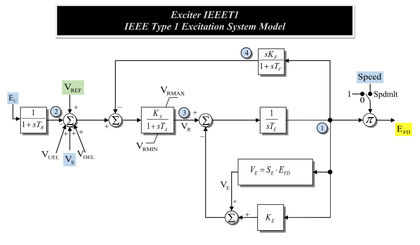
Figure 1: Exciter IEEET1 model. Figure courtesy of PowerWorld

Model Parameters

Symbol	Units	Description	Typical Value
\(T_R\)	[sec]	Time constant for voltage sensing	0
\(K_A\)	[p.u.]	Coefficient for voltage regulation	50
\(T_A\)	[sec]	Time constant for voltage regulation	0.04
\(K_E\)	[p.u.]	Coefficient for excitation system	-0.06
\(T_E\)	[sec]	Time constant for excitation system	0.6
\(K_F\)	[p.u.]	Coefficient for feedback	0.09
\(T_F\)	[sec]	Time constant for feedback	1.46
\(V_R^{\min}\)	[p.u.]	Lower limit to voltage regulation	-1
\(V_R^{\max}\)	[p.u.]	Upper limit to voltage regulation	1
\(E_1\)	[p.u.]	Saturation Parameter	2.8
\(E_2\)	[p.u.]	Saturation Parameter	3.73
\(S_1\)	[p.u.]	Saturation Parameter	0.04
\(S_2\)	[p.u.]	Saturation Parameter	0.33
\(I_{\mathrm{spdlim}}\)	[binary]	Speed limit flag indicator	0

Parameter Validation

Invalid IEEET1 parameter sets are rejected by the following checks. Let \(\epsilon_T=10^{-3}\).

\[\begin{split}\begin{aligned} T &\leftarrow \max\!\left(T, \epsilon_T\right) \quad T \in \{T_R, T_A, T_E, T_F\} \\ K_A &> 0 \\ V_R^{\min} &\le V_R^{\max} \\ I_{\mathrm{spdlim}} &\in \{0,1\} \\ \left(S_1, S_2\right) &=(0,0) \quad\text{or}\quad \begin{gathered} E_1, E_2, S_1, S_2 > 0 \\ E_1 \ne E_2 \\ S_1 \ne S_2 \end{gathered} \end{aligned}\end{split}\]

Model Derived Parameters

When saturation is disabled, \(S_A=0\) and \(S_B=0\). Otherwise, the parameters are chosen so that the following quadratic model represents the expected saturation near the operating region:

\[\begin{split}\begin{aligned} S_1 &= S_B(E_1-S_A)^2 \\ S_2 &= S_B(E_2-S_A)^2 \\ \end{aligned}\end{split}\]

Generally, this system has two solutions. The non-extraneous solution is as follows.

\[\begin{split}\begin{aligned} C &= \sqrt{ \dfrac {S_2} {S_1} } \\ S_A &= \dfrac {C E_1 - E_2} {C - 1} \\ S_B &= \dfrac {S_1} {(E_1-S_A)^2} \end{aligned}\end{split}\]

Model Variables

Internal Variables

Differential

Symbol	Units	Description
\(V_{ts}\)	[p.u.]	Sensed terminal voltage
\(V_R\)	[p.u.]	Voltage regulator
\(E_{fd}'\)	[p.u.]	Field-current pre-speed multiplier
\(V_{fx}\)	[p.u.]	Exciter feedback internal state

Algebraic

Symbol	Units	Description
\(V_{tr}\)	[p.u.]	Terminal Voltage Error
\(V_f\)	[p.u.]	Feedback Voltage
\(V_E\)	[p.u.]	Excitation control voltage
\(E_{fd}\)	[p.u.]	Field winding voltage
\(k_\text{sat}\)	[p.u.]	Saturation variable

External Variables

Symbol	Units	Description	Note
\(V_r\)	[p.u.]	Real bus voltage component
\(V_i\)	[p.u.]	Imaginary bus voltage component
\(V_\text{ref}\)	[p.u.]	Reference terminal voltage
\(V_{UEL}\)	[p.u.]	Input from under excitation limiter	Constant zero until modeled
\(V_{OEL}\)	[p.u.]	Input from over excitation limiter	Constant zero until modeled
\(V_S\)	[p.u.]	Input from stabilizer controller	Optional, defaults to zero
\(\omega\)	[p.u.]	Machine speed deviation	Optional, defaults to zero

Model Equations

Differential Equations

For readability, define the pre-limit derivative of \(V_R\) and voltage-sensing input:

\[\begin{split}\begin{aligned} f_R &:= \dfrac{1}{T_A}\left(-V_R + K_A V_{tr}\right) \\ E_C &:= \sqrt{V_r^2 + V_i^2} \end{aligned}\end{split}\]

The IEEET1 differential equations, as derived from the model diagram, are:

\[\begin{split}\begin{aligned} 0 &= -\dot V_{ts} + \dfrac{1}{T_R}\left(E_C - V_{ts}\right) \\ 0 &= -\dot V_R + \text{antiwindup} \left(V_R, f_R; V_R^{\min}, V_R^{\max}\right) \\ 0 &= -\dot E_{fd}' + \dfrac{1}{T_E}\left(V_R - V_E - K_E E_{fd}'\right) \\ 0 &= -\dot V_{fx} + \dfrac{1}{T_F}\left(V_f\right) \end{aligned}\end{split}\]

CommonMath defines the smooth Anti-Windup target and approximation.

Algebraic Equations

The algebraic equations of the exciter.

\[\begin{split}\begin{aligned} 0 &= -V_{ts} + V_\text{ref} + V_{UEL} + V_{OEL} + V_S - V_{tr} - V_f \\ 0 &= -T_F(V_f + V_{fx}) + K_F E_{fd}' \\ 0 &= -V_E + k_\text{sat} E_{fd}' \\ 0 &= -E_{fd} + (1 + \omega I_{\mathrm{spdlim}})E_{fd}' \\ 0 &= -k_\text{sat} + S_B\, q(E_{fd}' - S_A) \end{aligned}\end{split}\]

Here \(q\) is GridKit’s Quadratic Ramp.

Initialization

The implementation first applies \(T \leftarrow \max(T, 10^{-3})\) for \(T \in \{T_R, T_A, T_E, T_F\}\). This should be replaced with a structural template change in the future. The machine initializes \(E_{fd}\) first. IEEET1 reads that value as \(E_{fd,0}\), along with any attached \(\omega\) and \(V_S\), and solves the steady-state algebraic chain so all residuals vanish with \(\dot y = 0\). The sensed terminal voltage initializes from the positive bus-voltage magnitude. Saturation is included when enabled, and the speed-limit flag is included directly; \(V_\text{ref}\) is set to close the \(V_{tr}\) equation with the current input values.

\[\begin{split}\begin{aligned} E_{C,0} &:= \sqrt{V_r^2 + V_i^2} \\ E_{fd}' &= \dfrac{E_{fd,0}}{1 + I_{\mathrm{spdlim}}\,\omega} \\ k_\text{sat} &= S_B\, q(E_{fd}' - S_A) \\ V_E &= k_\text{sat}\, E_{fd}' \\ V_R &= K_E\, E_{fd}' + V_E \\ V_{tr} &= \dfrac{V_R}{K_A} \\ V_{fx} &= \dfrac{K_F}{T_F}\, E_{fd}' \\ V_{ts} &= E_{C,0} \\ V_f &= 0 \\ V_\text{ref} &= E_{C,0} + V_{tr} - V_{UEL} - V_{OEL} - V_S \end{aligned}\end{split}\]

All internal derivatives initialize to zero.

Monitorable Variables

Variable	Units	Description	Note
`efd`	[p.u.]	Field winding voltage
`ksat`	[p.u.]	Magnetic saturation coefficient	\(S_B\,q(E_{fd}'-S_A)\)