Branch

Transmission lines and different types of transformers (traditional, Load Tap-Changing transformers (LTC) and Phase Angle Regulators (PARs)) can be modeled with a common branch model.

Transmission Line Model

The most common circuit that is used to represent the transmission line model is \(`\pi`\) circuit as shown in Figure 1. The nominal flow direction is from sending bus s to receiving bus r.

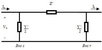
Figure 1: Transmission line \(`\pi`\) equivalent circuit

Here

\[Z'=R+jX\]

and

\[Y'=G+jB,\]

where \(`R`\) is line series resistance, \(`X`\) is line series reactance, \(`B`\) is line shunt charging, and \(`G`\) is line shunt conductance. As can be seen from Figure 1 total \(`B`\) and \(`G`\) are separated between two buses. The current leaving the sending bus can be obtained from Kirchhoff’s current law as

\[I_s = y(V_s - V_r) + \frac{Y'}{2} V_s,\]

where \(`V_s`\) and \(`V_r`\) are voltages on sending and receiving bus, respectively, and

\[y = \frac{1}{Z'} = \frac{R}{R^2+X^2} + j\frac{-X}{R^2+X^2} = g + jb.\]

Similarly, current leaving receiving bus is given as

\[-I_R = y(V_r - V_s) + \frac{Y'}{2} V_r.\]

These equations can be written in a compact form as:

\[\begin{split}\begin{bmatrix} I_{s}\\ -I_{r} \end{bmatrix} = \mathbf{Y}_{TL} \begin{bmatrix} V_{s}\\ V_{r} \end{bmatrix}\end{split}\]

where:

\[\begin{split}\mathbf{Y}_{TL}=\begin{bmatrix} g + jb + \dfrac{G+jB}{2} & -(g + jb) \\ -(g + jb) & g + jb + \dfrac{G+jB}{2} \end{bmatrix}\end{split}\]

Branch contributions to residuals for sending and receiving bus

Complex power leaving sending and receiving bus is computed as

\[\begin{split}\begin{bmatrix} S_{s}\\ S_{r} \end{bmatrix} = \begin{bmatrix} V_{s}\\ V_{r} \end{bmatrix} \begin{bmatrix} I_{s}\\ -I_{r} \end{bmatrix}^* = \begin{bmatrix} V_{s}\\ V_{r} \end{bmatrix} \mathbf{Y}_{TL}^* \begin{bmatrix} V_{s}\\ V_{r} \end{bmatrix}^*\end{split}\]

After some algebra, one obtains expressions for active and reactive power that the branch takes from adjacent buses:

\[P_{s} = \left(g + \frac{G}{2}\right) |V_{s}|^2 + [-g \cos(\theta_s - \theta_r) - b \sin(\theta_s - \theta_r)] |V_{s}| |V_{r}|\]

\[Q_{s} = -\left(b + \frac{B}{2}\right) |V_{s}|^2 + [-g \sin(\theta_s - \theta_r) + b \cos(\theta_s - \theta_r)] |V_{s}| |V_{r}|\]

\[P_{r} = \left(g + \frac{G}{2}\right) |V_{r}|^2 + [-g \cos(\theta_s - \theta_r) + b \sin(\theta_s - \theta_r)] |V_{s}| |V_{r}|\]

\[Q_{r} = -\left(b + \frac{B}{2}\right) |V_{r}|^2 + [ g \sin(\theta_s - \theta_r) + b \cos(\theta_s - \theta_r)] |V_{s}| |V_{r}|\]

These quantities are treated as loads and are substracted from \(`P`\) and \(`Q`\) residuals computed on the respective buses.

Branch Model

Note: Transformer model not yet implemented

The branch model can be created by adding the ideal transformer in series with the \(`\pi`\) circuit as shown in Figure 2 where \(`\tau`\) is a tap ratio magnitude and \(`\theta_{shift}`\)is the phase shift angle.

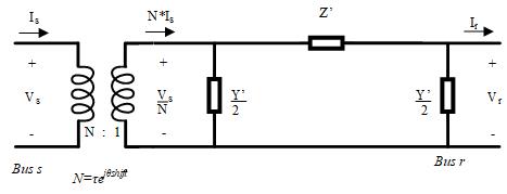
Figure 2: Branch equivalent circuit

The branch admitance matrix is then:

\[\begin{split}\mathbf{Y}_{BR}= \begin{bmatrix} \left(g + jb + \dfrac{G+jB}{2} \right)\dfrac{1}{\tau^2} & -(g + jb)\dfrac{1}{\tau e^{-j\theta_{shift}}}\\ &\\ -(g + jb)\dfrac{1}{\tau e^{j\theta_{shift}}}. & g + jb + \dfrac{G+jB}{2} \end{bmatrix}\end{split}\]

Branch contribution to residuals for sending and receiving bus

The power flow contribution for the transformer model are obtained in a similar manner as for the \(`\pi`\)-model.